Task 3 — MPI | EdgeGuard SS2026

What is MPI?

MPI (Message Passing Interface) is the standard for parallel programming on distributed memory systems. Each MPI process runs independently on its own memory — processes communicate explicitly by sending and receiving messages over the network. We used OpenMPI deployed across all 8 Pi3 nodes, giving us 32 MPI processes (4 cores × 8 nodes).

The key insight MPI reveals is that communication overhead determines parallel scalability. An algorithm with minimal communication scales near-ideally. An algorithm that must send large amounts of data between processes hits a ceiling — no matter how many cores you add.

Test Setup

Pre-Benchmark Checklist

bashRun before every MPI benchmark

# 1. Stop k3s-agent on all Pi3 nodes
for ip in 10.10.10.21 10.10.10.22 10.10.10.23 10.10.10.24 \
          10.10.10.25 10.10.10.26 10.10.10.27 10.10.10.28; do
    ssh admin@$ip "sudo systemctl stop k3s-agent" &
done
wait

# 2. Check temperatures (should be below 65°C)
for ip in 10.10.10.21 10.10.10.22 10.10.10.23 10.10.10.24 \
          10.10.10.25 10.10.10.26 10.10.10.27 10.10.10.28; do
    echo -n "$ip: "
    ssh admin@$ip "vcgencmd measure_temp"
done

# 3. Kill any leftover MPI processes
for ip in 10.10.10.21 10.10.10.22 10.10.10.23 10.10.10.24 \
          10.10.10.25 10.10.10.26 10.10.10.27 10.10.10.28; do
    ssh admin@$ip "pkill -f monte_carlo_pi; pkill -f matrix_multiply" 2>/dev/null
done

MPI Hostfile

The hostfile defines which nodes and how many cores per node participate. We used a Pi3-only hostfile — Pi5 was always excluded from MPI compute.

text~/mpi_hosts_pi3only

pi3-01 slots=4
pi3-02 slots=4
pi3-03 slots=4
pi3-04 slots=4
pi3-05 slots=4
pi3-06 slots=4
pi3-07 slots=4
pi3-08 slots=4

Two MPI Examples

We chose two examples with contrasting communication patterns to clearly demonstrate how communication complexity determines parallel scalability.

Example 1

Monte Carlo Pi

Each MPI rank independently generates random points and checks if they fall inside a unit circle. A single MPI_Reduce at the end combines all counts to estimate π.

Communication: O(1) — one MPI_Reduce regardless of N Type: Embarrassingly parallel Problem sizes: 0.1M, 1M, 10M, 100M, 1B, 10B points Core counts: 1, 2, 4, 8, 16, 32 Runs: 3–5 per configuration

Example 2

Matrix Multiplication

Dense matrix C = A × B. Each rank receives rows of A via MPI_Scatter and a full copy of matrix B via MPI_Bcast. Results gathered with MPI_Gather.

Communication: O(N²) — MPI_Bcast sends full matrix B Type: Dense parallel — communication grows with N Problem sizes: N=1000, 1500, 2000, 3000, 3250, 3500, 3750, 4000 Core counts: 1, 2, 4, 8, 16, 32 Runs: 5 per configuration

ℹ️ Why these two examples?

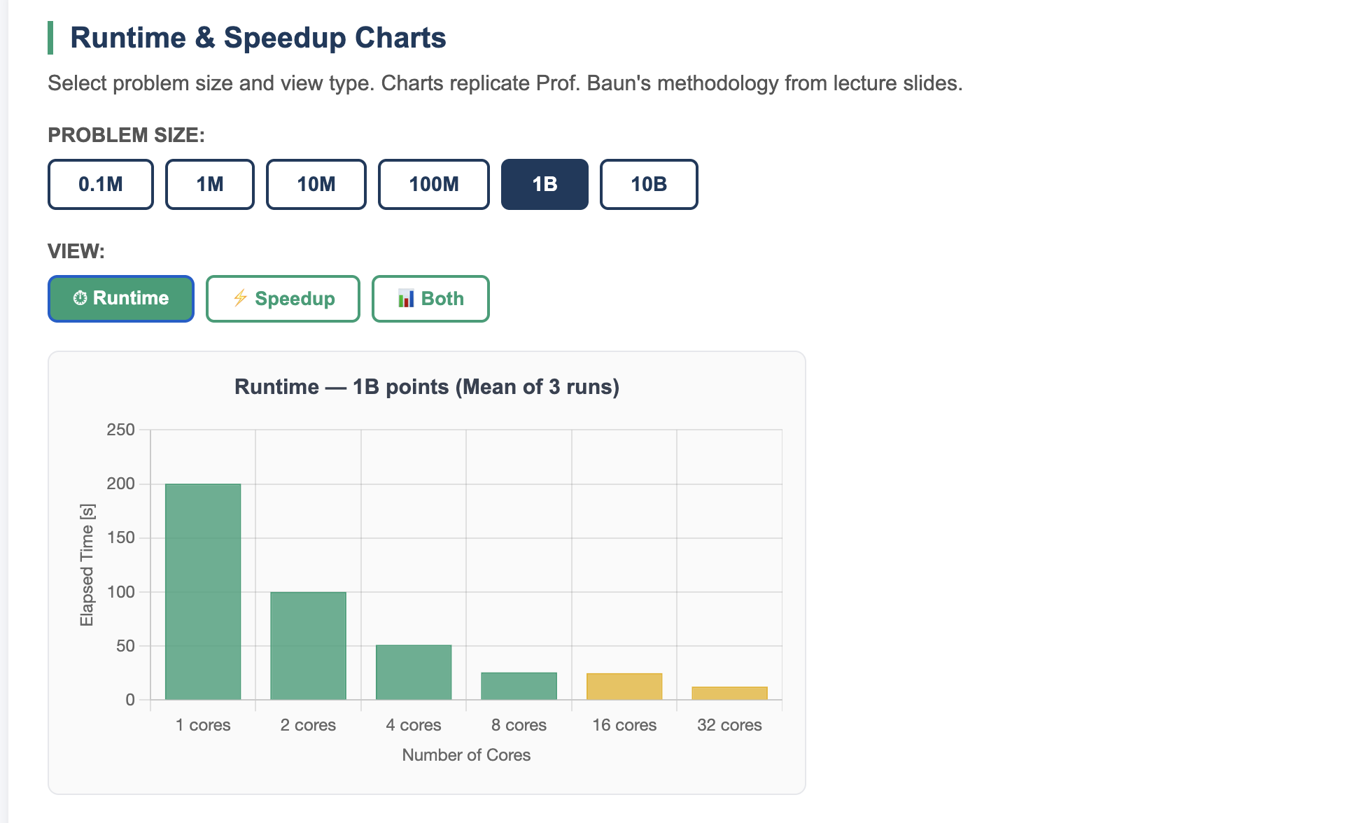
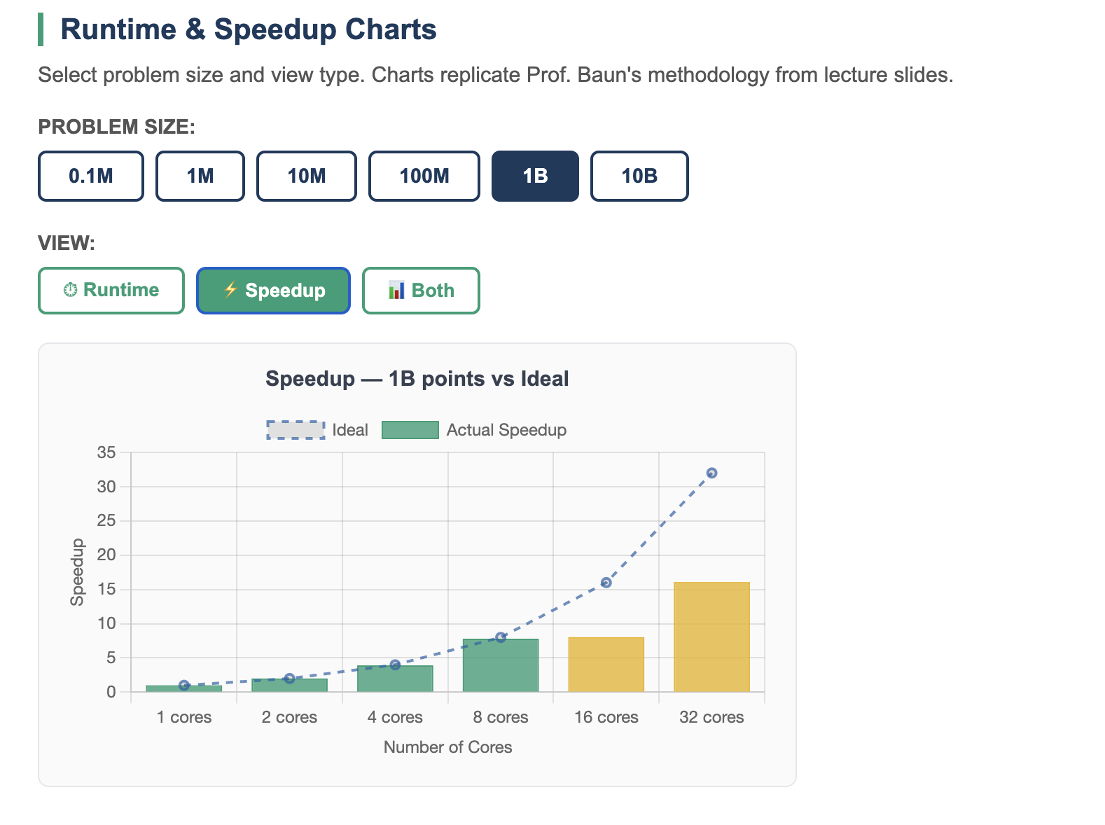
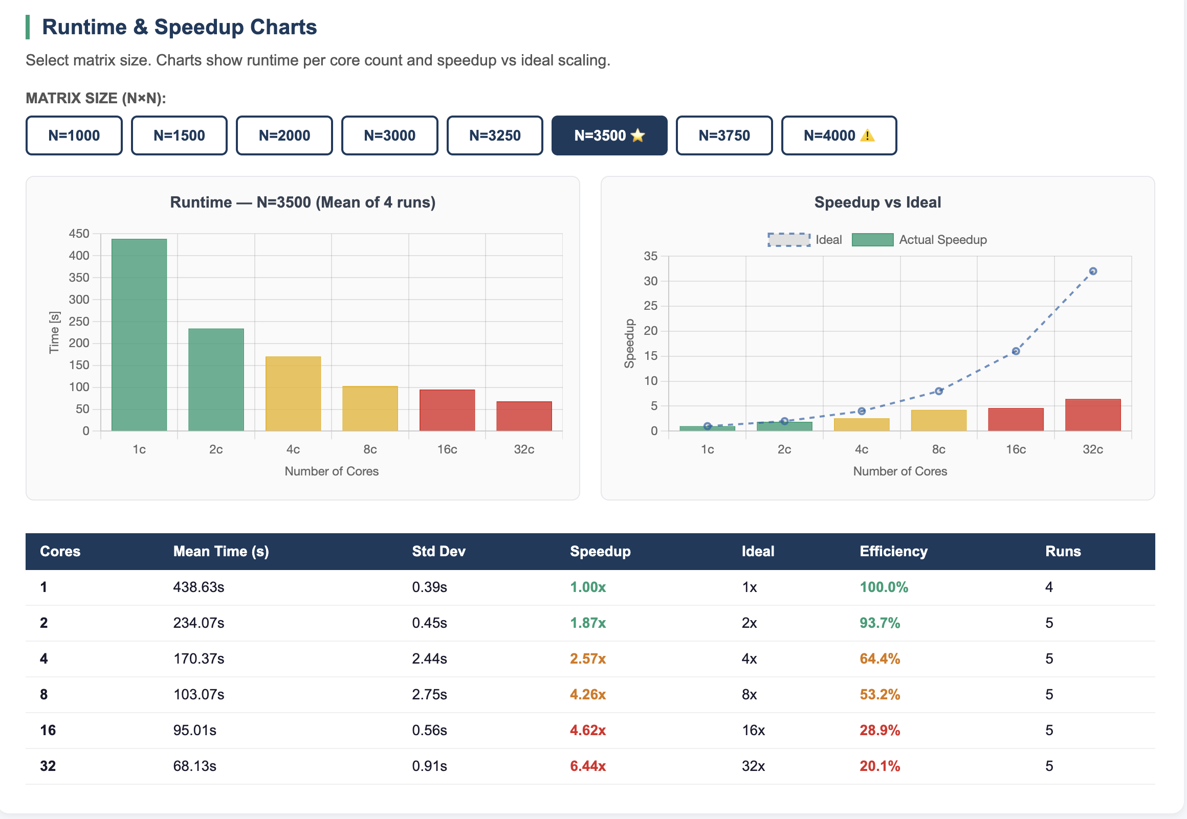
The contrast is intentional. Monte Carlo Pi has O(1) communication and achieves 16.2× speedup at 32 cores. Matrix Multiplication has O(N²) communication and achieves only 6.41× at 32 cores. This directly demonstrates how communication pattern determines the parallelization limit — the core insight behind both Amdahl's and Gustafson's Laws.

How to Reproduce

Monte Carlo Pi

bashRun Monte Carlo Pi

# Binary location: ~/monte_carlo_pi
# Replace <CORES> with: 1, 2, 4, 8, 16, or 32
# Replace <POINTS> with: 100000, 1000000, 10000000,
#                         100000000, 1000000000, 10000000000

mpirun -np <CORES> \
    --hostfile ~/mpi_hosts_pi3only \
    ~/monte_carlo_pi <POINTS>

# Example: 32 cores, 1 billion points
mpirun -np 32 --hostfile ~/mpi_hosts_pi3only ~/monte_carlo_pi 1000000000

# Output: <time_seconds> <pi_estimate> <cores> <points>
# Example: 12.566 3.14159 32 1000000000

Matrix Multiplication

bashRun Matrix Multiplication

# Binary location: ~/matrix_multiply
# Replace <CORES> with: 1, 2, 4, 8, 16, or 32
# Replace <N> with: 1000, 1500, 2000, 3000, 3250, 3500, 3750, or 4000
# Note: N=5000 causes memory swap on Pi3 — avoid

mpirun -np <CORES> \
    --hostfile ~/mpi_hosts_pi3only \
    ~/matrix_multiply <N>

# Example: 8 cores, N=3500 (sweet spot)
mpirun -np 8 --hostfile ~/mpi_hosts_pi3only ~/matrix_multiply 3500

# Output: <time_seconds> <N> <cores>

⚠️ Memory limit for Matrix Multiply

Each MPI process holds a full copy of matrix B in memory (N² × 8 bytes). At N=5000 this causes memory swap on Pi3 nodes (confirmed: 470MB swap usage). Maximum safe N is 3500–4000. Sweet spot is N=3500 — best scaling without memory pressure.

Amdahl's Law & Gustafson's Law

Both scaling laws are demonstrated across our two MPI examples. Full charts and analysis are in the Results page.

Amdahl's Law — Fixed Problem Size

Speedup is limited by the serial fraction of the program. No matter how many cores you add, the serial part (communication overhead) creates a ceiling.

Visible in Monte Carlo Pi at 0.1M points: 1 core = 0.020s, 32 cores = 0.240s — adding cores makes it SLOWER because MPI_Reduce overhead dominates the trivial 0.0006s compute time.

Gustafson's Law — Scaled Problem Size

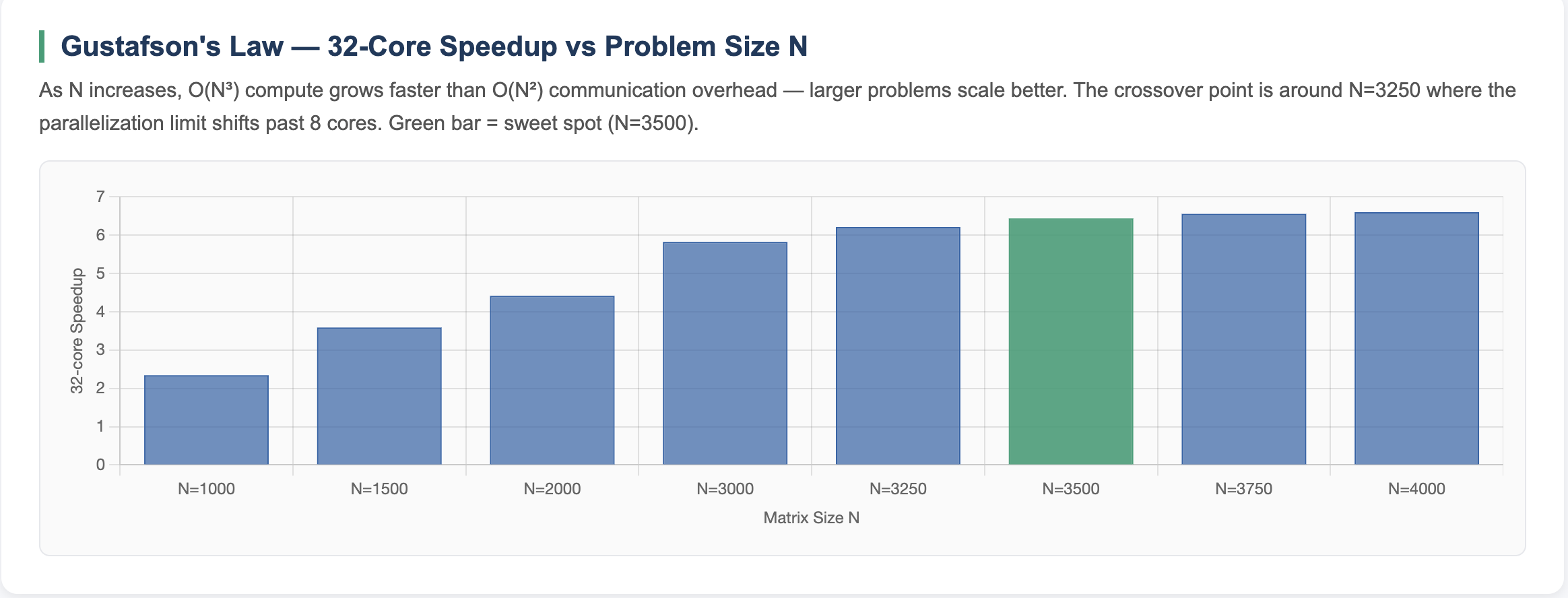
If you increase the problem size proportionally with the number of cores, the parallel fraction grows and efficiency improves — the serial fraction becomes relatively smaller.

Visible in Monte Carlo Pi: at 1M points → 5.1× speedup at 32 cores. At 10B points → 16.2× speedup at 32 cores. Same hardware, bigger problem = better scaling.

📊 mpi_amdahl_gustafson.png Speedup vs Core Count — All Problem Sizes (Monte Carlo Pi)

Figure 1 — Speedup curves for all problem sizes. Small N (Amdahl) collapses quickly. Large N (Gustafson) approaches ideal.

Results — Chart Overview

Detailed results with min/max/mean tables and interactive charts are on the Results page. Key chart previews below.

Monte Carlo Pi

⏱️ monte_carlo_runtime.png Runtime vs Cores — All Problem Sizes

⚡ monte_carlo_speedup.png Speedup vs Cores — All Problem Sizes

Matrix Multiplication

📈 matrix_speedup_n3500.png Speedup vs Cores — N=3500 (sweet spot)

📊 matrix_speedup_vs_n.png 32-Core Speedup vs Problem Size N (Gustafson)

Key Findings

✅ Monte Carlo Pi — 16.2× speedup at 32 cores (10B points)

O(1) communication allows near-ideal scaling at large problem sizes. The parallelization limit is at 8 cores — caused by network topology when crossing from 2 to 4 physical nodes, not by problem size.

✅ Matrix Multiply sweet spot — N=3500, 6.41× at 32 cores

O(N²) communication limits scaling. Parallelization limit shifts from 4 cores (N=1000) to 8 cores (N=1500) to broken at N=3250 — demonstrating Gustafson's Law: larger problem = limit pushed further.

⚠️ Parallelization limit at 8 cores (2 nodes)

In Monte Carlo Pi, 8→16 cores provides less than 3% improvement regardless of problem size (tested 1B to 25B points). The limit is structural — crossing from 2 to 4 physical nodes introduces network overhead that dominates the MPI_Reduce.